Automating the selection of genome assembly software
The selection of the optimal assembler an important part of processing genomic data, where each assembly represents a hypothesis as to the best way to reconstruct a genome from the sequencing reads. An open question is what is the best way to determine if the produced assembly is good, and by what criteria? Previous approaches including the Assemblathon 1 [1], Assemblathon 2 [2], GAGE [3], and CAMI [4] have surveyed the different available assembly methods.
The “nucleotid.es” project is an automated benchmarking framework to examine short read assembly software. The aim of automating benchmarking was to have an always up-to-date overview of the current state of efficacy, performance, and correctness for genome assembly software. The testing data included 16 different microbial genomes, where each source organism had five technical replicates generated by sampling without replacement from a superset of reads. Each assembler was then benchmarked against a total of 80 FASTQ files. All the microbial sources used are listed in Table 9. None of the sequencing data used were preprocessed by any tools prior to assembly, and can be considered as ‘raw’ Illumina sequencing data. Though not recommended practice, this simplified the analysis by allowing comparison of assembly pipelines containing preprocessing steps.
Examining a data set containing a variety of different microbial genomes allows estimating confidence intervals, and ideally the identification of small differences in assembler efficacy. As the JGI sequences thousands of microbial genomes, even a small improvement in assembly quality could result in thousands of additional correct genome features. To this end ‘nucleotid.es’ collected 5.6 million metrics across 18.57 million assembled contigs, using a combined total of approximately 8.8k CPU hours.
This automated benchmarking approach was made possible through the use of Docker images with standardised interfaces to the majority of recent genome assembly software, via the bioboxes project [5] developed in conjunction with Peter Belmann and our other CAMI collaborators. The use of bioboxes increases the utility of the performance metrics to be useful to the microbial genomics community, since researchers can download and use exactly the same Docker image in their own work as was benchmarked here.
The metrics were generated using QUAST 4.5 and an internally-develop JGI tool: GAET. QUAST is described in Gurevich et. al 2013 [6], while GAET compares a reference genome and an assembly by looking at the differences in the two respective annotation sets. The assemblers compared in this analysis were ABySS [7], A5-miseq [8], GATB Minia [9], LightAssembler [10], MEGAHIT [11], Ray [13], Shovill, SPAdes [14], StriDe [15], BBTools Tadpole, Unicycler [16], and Velvet [17]. The isolate assembly pipeline being used in production at the JGI was also included in the analysis. This pipeline is several preprocessing steps using BBTools followed by assembly with SPAdes. All the versions of each short read assembler Docker image used in this analysis are listed in Table 8.
Many different approaches have been used to examine and define genome quality [18], [19], [20], [21], [22], [23], [24], [25]. There is no consensus within the bioinformatics community on what a single unified assembly quality metric. This analysis instead compares assemblers using the several quality metrics that have been commonly used previously. Furthermore all the ‘nucleotid.es’ data generated here are available for download so that anyone may also do their own assessment, according to which assembly metrics are most useful to their own work. This data set contains 100s of metrics per assembly based on comparing a set of contigs as the “observed” assembly against a reference sequence as the “expected” genome using both QUAST and GAET . The analysis presented here is also an RMarkdown document containing all the R code used. You can view the source or submit a pull request through the gitlab repository.
Modelling genome assembler efficacy
The aim of generating the ‘nucleotid.es’ data was to estimate the efficacy of each assembler. As each assembler was benchmarked across multiple different genomes, any estimate for assembler efficacy needed to account for some genomes being more difficult to assemble than others. Any estimate should be an aggregate across all assessed genomes while holding any genome-specific differences constant.
To this end, linear models were used to estimate two different coefficients, one for each assembler, and one for each genome. As an example the NA50 value of any given genome assembly was split into two components: the first component measured the overall difficulty of assembling the genome, such as might be limited by genomic repeats. The second component measured the assembler efficacy, where given the same input data, each assembler produces more or less contiguous assemblies.
Equation 1 shows an example where NA50 is the sum of the estimated coefficients for two components plus any error unaccounted for in the model, using SPAdes and E. coli. In this equation, the model estimated value for \(\beta_1\) represents the efficacy of an assembler holding the differences in genome \(\beta_2\) constant. This value, along with the associated confidence intervals, was used as a measure for assembler efficacy. The natural logarithm of the genome length (\(ln. length\)) was included to account for differences in genome length. Using a log-link function for the linear model means that changes in the estimated explanatory coefficients have a log. normal change in the response variable.
\[\begin{align} \begin{split} \frac{metric}{length} & = exp. \left(\beta_1 \cdot assembler + \beta_2 \cdot genome \right) + \epsilon \\ \\ metric & = exp. \left(\beta_1 \cdot assembler + \beta_2 \cdot genome + 1 \cdot ln.\ length \right) + \epsilon \\ \\ NA50 & = exp. \left(-3.196 \cdot SPAdes + -0.30781 \cdot E.coli + 1 \cdot 15.35 \right) + - 6890 \\ & = 139,552\ bp \\ \end{split} \tag{1} \end{align}\]We wanted to use model fitting to measure genome assembler efficacy, accounting for noise and differences in genomes, however it was not clear a priori which model to use. Selecting a model ourselves could introduce biases based on our own intuitions about what the most accurate model should be. The ideal scenario was to allow the data to inform us as to which model to use. Therefore, the first step in this analysis was to test different mixed-effect linear models1 to determine which best describes genome assembler efficacy. The aim was to compare different hypotheses, including the null, and select the most parsimonious given the data.
The Bayesian information criterion (BIC) was used to rank to each model, where BIC is the log-likelihood of the model penalised by the number of free parameters, multiplied by number of data points. The model with the lowest BIC was the one selected as the most parsimonious - that which best fits the data without overfitting by using too many parameters.2 The models tested to explain the variance in assembles are listed in Table 6.
Random slopes were not considered as all the dependent variables were categorical. Each model had a random effect intercept fitted. Each random intercept was fitted for the terms described below.
-
Null - No random intercept terms were fitted.
-
Genome - A different random intercept coefficient was fitted for each source genome term.
-
FASTQ file - A different random intercept coefficient was fitted for each FASTQ file term.
These random intercepts allowed for each model to account for genome or input file differences in the data that were not specific to the assembler. Each model also had four variations in fixed-effect explanatory variable. These were:
-
Null - assembly quality is random regardless of which assembler is used.
-
Assembler - the explanatory effect for assembly quality is the assembler used, regardless of the version or command line arguments.
-
Assembler Version - the explanatory effect for assembly quality is the version of the assembler used, regardless of command line arguments.
-
Assembler Args - the explanatory effect for assembly quality is the command line arguments for that version of the assembler used.
The “Fixed Effect” and “Random Effect” components allowed for fitting different coefficients (\(\beta_1, \beta_2\)) averaged across the data. This was suitable for measuring single point-estimates, however we also wanted to estimate 95% confidence intervals for each assembler. Confidence intervals allowed comparing each assembler conservatively using the expected worst-case result. I.e. instead of comparing by the mean performance of each assembler, compare by the lower 5% confidence interval.
In addition to estimating mean coefficients for each genome or assembler, different variances were considered too. This modelled whether the efficacy of one assembler had a wider range of results than another. These variance components are listed in the ‘Variance Model’ column of Table 6. Each row lists which term was used to estimate a coefficient for the variance. Null indicates a single global term was estimated for the entire model, i.e. a mixed-effect model with no specific modelling of variance.
Example model fitting for contiguity
As an example, model fitting and comparison was performed by fitting each these model using NA50 as the explanatory variable. Figure 1 shows the distribution of NA50 values scaled by the length of the source genome. NA50, a metric used to assess assembly quality based on contiguity, is defined as the contig length where the cumulative sum of the ordered contigs lengths in the assembly was at least half the total assembly length, removing any contigs that don’t align to the reference sequence. Scaling NA50 by the reference length controls for the size of the genome when comparing assemblies from two different source organisms. This becomes a unitless metric between 0-1, where 1 represents an assembly without any gaps.
Figure 1 shows that scaled NA50 is distributed across four orders of magnitude from \(10^{-3} - 10^{0}\), and is variable both between organisms and within the same organism. The figure highlights that assembly quality appears to be highly dependent on the organism being sequenced, even when accounting for the differences in the length of the source organism using the \(ln. length\) term in Equation 1. This effect is modelled by the \(\beta_2\) component in Equation 1, the per-organism variability in assembly quality. In the case of contiguity, this is likely due to the repeat content of the genome and short read length [28]. The effect of GC content or number of repeats in the genome were not considered, all these factors would instead be lumped into the single genome-specific term.
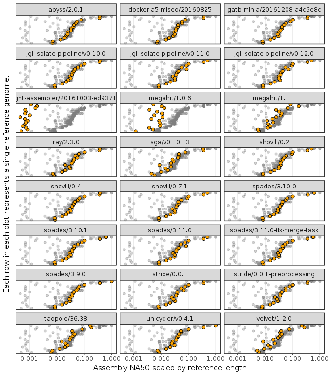
Figure 1: Plot of NA50 distribution across genome assembler version. The x-axis is NA50 scaled by source genome length, shown on a log. scale. The rows on the y-axis are the benchmark genomes ordered by the geometric mean across all assemblies. Each facet plot shows all the different assembly values across all assemblers in grey, with the specific values for that assembler highlighted. Organism labels are hidden for brevity.
| Fixed Term | Random Term | Variance Model | dBIC | R.D.F. | Dev. | Conv. |
|---|---|---|---|---|---|---|
| Assembler Args | Genome | Assembler Args + Genome | 0.00 | 3627.001 | 82812.7 | T |
| Assembler Args | Input FASTA | Assembler Args + Input FASTA | 967.93 | 3499.019 | 82727.2 | T |
| Assembler Version | Genome | Assembler Version + Genome | 1674.87 | 3677.001 | 84899.1 | T |
| Assembler | Genome | Assembler + Genome | 2134.88 | 3697.001 | 85523.8 | T |
| Assembler Args | Genome | Assembler Args | 2160.55 | 3642.001 | 85096.7 | T |
| Assembler Version | Input FASTA | Assembler Version + Input FASTA | 2656.14 | 3549.027 | 84827.0 | T |
Table 1: Summary of first six most parsimonious models with NA50 as the response variable. The dBIC shows the difference in Bayesian information criterion between the best model and all other models. ‘R.D.F.’ is the residual degrees of freedom in the model. ‘Dev.’ is the residual deviance in the model. ‘Conv.’ states whether the model converged or not (T/F).
All the models described (Table 6) were fitted with NA50 as the response variable. The best five models according to lowest BIC are listed in Table 1. This table shows the dBIC, residual deviance, and residual degrees of freedom for each model.3 The dBIC value shows the delta between each model and the model with the lowest BIC. Therefore the most parsimonious model for explaining variance in NA50, according to BIC, was assembler command line arguments with a random effect for source genome and variance components for both assembler arguments and genome. The next most parsimonious model had a dBIC much higher than 10, indicating there is no support for it or any other models [29].
As an aside, the null model with only the random effect for source organism was more parsimonious compared with the subset of models using only software as an explanatory effect without a random effect for source genome(not shown in the table for clarity). This emphasises the importance considering the biological source when benchmarking bioinformatics software, and any performance metrics must account for inherent random effects in the benchmark data used. The model comparison suggests not accounting for this is likely to conflate the efficacy of the software with the inherent differences in the data used for benchmarking.
Examining assembly metrics
Contiguity metrics such as NA50, count only the contigs that align to the reference. In addition to NA50, misassemblies, indels, mismatches, and Ns are regularly used to examine the quality of an assembly. These other metrics are useful to describe an assembly because incorrect regions in assemblies are likely to be annotated incorrectly, which can then subsequently change downstream analysis of the genomic features in these erroneous regions.
The above modelling approach used to examine NA50 was also applied to the number of misassemblies, and the number of incorrect bases in the same assemblies determined by aligning to the reference. The number of incorrect bases was defined as the sum of indels, mismatches and Ns. The estimated assembler coefficients (\(\beta_1\) in Equation 1) from the most parsimonious model in each case are shown in Figure 2. These assembler coefficients are point estimates with 95% confidence intervals from a log-normal distribution.4 The assemblers are ranked by the worst bound on the confidence intervals, which is the lower bound in the case of NA50 and the upper bound for number of misassemblies, and incorrect bases. In the cases where multiple different command line arguments for the same version were tested, the assemblers were ranked by the command line arguments that gave the “least-worst” coefficient by confidence interval. The least-worst was determined by ranking all the command line parameter sets within the same tool version, and selecting the set with the highest lower bound on the estimated coefficient confidence intervals. Ranking by least-worst on the lower bound of the confidence interval estimates was because assemblers with large confidence intervals could generate both very good and very poor results. Using the lower bound ranks assemblers by the worst-case expected result.
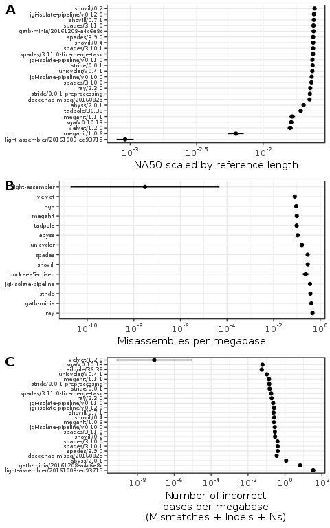
Figure 2: Plot of assembly quality metrics by genome and assembler. Each figure shows the efficacy of the assembler coefficients estimated from a linear model accounting for both the genome and the assembler software used. The error bars show the 95\% confidence intervals for each estimate. The x-axis for the model coefficient plots are ordered by the least-worst bound on the confidence interval for each assembler. Figures A and C include the different versions of the assembly software used. Figure B does not include the assembly software version because the most parsimonious model indicated software version is not a factor in rate for the assemblers and versions tested.
Figure 2A shows the linear-model estimated NA50 coefficient for each assembler, the model coefficients are exponentiated to appear on 0-1 scale as NA50 scaled by reference genome length. The estimated coefficients show that the choice of genome assembler had a relatively minor effect on the contiguity of the assembly, where most assemblers can be expected to produce similar contiguity. The exceptions to this are LightAssembler and MEGAHIT/1.0.6. MEGAHIT versions 1.0.6 and 1.1.1 have different estimates with non-overlapping confidence intervals, highlighting the important of considering and reporting which version of an assembler was used in any genomic analysis. Overall though the choice of assembler appears to have only a minor affect on contiguity.
Figure 2B shows the estimated average misassembly coefficients for each genome assembler, exponentiated to return to the original scale. The estimated coefficients are more uniformly distributed across a range of values than the estimated NA50 coefficients. In this case there are assemblers such as LightAssembler, tadpole and MEGAHIT that generate fewer misassemblies than assemblers such as Ray, Minia, StriDe and the JGI isolate pipeline. The assemblers that have the largest coefficients for NA50, also tend to have the largest coefficients for misassemblies per megabase, indicating an positive relationship between contiguity and misassemblies.
Comparing the estimated coefficients for incorrect bases per megabase in Figure 2C shows that LightAssembler and Minia tend to generate larger numbers of incorrect bases, while all the other assemblers tend to produce much lower values.
In two metric plots, two of the assemblers velvet and LightAssembler had a small estimated coefficients with a large confidence interval range. This may indicate model difficulty in estimating accurate coefficients, which could be due to both of these assemblers failing to produce results for some benchmarks (Table 7). To put this another way, the worst results for both assemblers produced no assemblies at all, which could skew the data. Future analysis could develop an unbiased method of handling missing data.
For contiguity the most parsimonious model indicates that assembler arguments are relevant (Table 1), for misassemblies the most parsimonious model indicates that only the assembler is relevant regardless of version or assembler arguments (Table 3), and for incorrect bases the most parsimonious model indicates only the assembler version is relevant (Table 4).
Effect of assembler choice on annotations
The NA50, misassemblies and incorrect bases metrics all measure different components of assembly quality. Assemblies with better values for these metrics should be more representative of the true genome sequence. As mentioned earlier, an outstanding issue is the lack of a single metric to determine which genome assembly software to use. As an example of this are the results in Figure 2A and 2B indicate that optimising for contiguity is likely to increase misassembly rate, and vice versa. The ideal case is a single metric which may be used as an objective function not only for selecting assembly software, but also for making other optimisations, such as to library and sequencing protocols. The ideal function would be a weighted combination of different metrics drawn from the requirements of the users of the pipeline, and representing different orthogonal axes of assembly quality.
All of the metrics examined so far are likely to affect the annotations in the assembly. A break in contiguity, a misassembly, or an incorrect base in a genome feature could result in no feature being annotated, or possibly worse a misannotation. Therefore using annotated genomic features may be a useful proxy for a single metric, combining multiple different metrics at once. This is an issue specifically raised by Florea et. al [24] where differences in cow genome assemblies result in thousands of predicted gene differences.
Annotation changes between assemblies can be estimated by comparing the difference between the genome feature sequences in the assembly and the reference sets5. This distance can be measured as the L1 norm of annotations. The L1 norm is the sum over the following function: for each distinct annotation in the superset of the assembly and the reference, 0 if the annotation appears in both the reference and the assembly, and 1 otherwise. The recently open sourced JGI tool GAET was developed to estimate this.
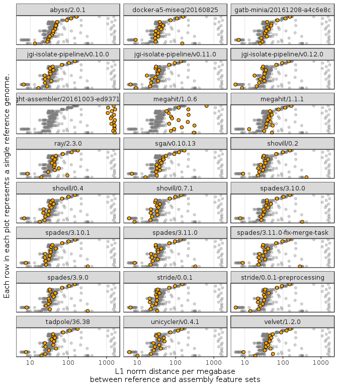
Figure 3: Plot of genome feature correctness by assembler version. The x-axis is the L1 norm distance of the annotated features between the assembly and the reference, shown on a log. scale. The rows on the y-axis are the benchmarked genomes ordered by the geometric mean across all assemblies. Each facet plot shows all the different assembly values across all assemblers in grey, with the specific values for that assembler highlighted. The y-axis is ordered by the geometric mean of values for each organism. Organism labels are hidden for brevity.
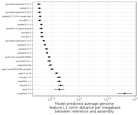
Figure 4: Plot of assembler average genome feature L1 norm distance coefficients. Coefficients were estimated from a linear model accounting for both the genome and the assembler software used. The error bars show the 95\% confidence intervals for each estimate. The x-axis is ordered by the lower bound on the confidence interval. The estimated coefficient for LightAssembler is not included on this scale due to it being much greater than all other estimated coefficients.
Figure 3 compares annotation L1 norm distance per megabase for all the genomes used in benchmarking, across all assemblers. The higher the L1 norm, the larger the difference between the reference and assembly annotated feature sets. In the majority of cases, the number of annotations different between the reference and the assembly is fewer than 200 per megabase, not including any genome specific effects. The exceptions to this were MEGAHIT/1.0.6 and LightAssembler which in many cases had a much larger number of differences compared with the other assemblers.
Similarly to the previous sections, the same models listed in Table 6 were fitted to describe the L1 norm distance between each assembly and the corresponding reference. The model for assembler with a random effect for source genome is the most parsimonious (Table 5). The again emphasises the importance of including the source genome when estimating software efficacy. Figure 4 shows the model estimated coefficients for the least-worst set of arguments for each assembler version. The figure shows that MEGAHIT/1.0.6 had higher number of incorrect annotations than the majority of the other assemblers, while this appears to be much improved in MEGAHIT/1.1.1. This again emphasises the importance of considering versioning in bioinformatics software. Light assembler could not be shown on the same scale as the other assemblers due to the estimated coefficient being much greater than the other assemblers. Outside of MEGAHIT/1.0.6 and LightAssembler the difference between the best and worst performing assembler was approximately 25 incorrect annotations per megabase. Therefore the choice of genome assembler is expected to have a non-trivial effect on downstream annotated features.
| Assembler | Version | Biobox Task | Estimate |
|---|---|---|---|
| jgi-isolate-pipeline | v0.11.0 | default | 52.99 |
| stride | 0.0.1 | default | 53.44 |
| jgi-isolate-pipeline | v0.12.0 | merge | 53.55 |
| shovill | 0.7.1 | default | 53.60 |
| spades | 3.11.0-fix-merge-task | merge | 53.59 |
| jgi-isolate-pipeline | v0.12.0 | experimental | 54.02 |
Table 2: List of five best performing assemblers by average L1 norm feature distance between the reference genome and the generated assembly. The ‘Assembler’, ‘Version’ and ‘Biobox Task’ columns refer to the parameters used to run the Docker image containing the software. The ‘Biobox Task’ refers to the biobox task name that can be used to replicate the command line arguments used for benchmarking. The ‘Estimate’ column is the upper 95% confidence interval on the average L1 norm distance across all the benchmark genomes. Larger values indicate an expected greater number of incorrect features in an assembly.
Table 2 lists the top five assembler biobox Docker images according the upper 95% confidence interval on the linear model estimated efficacy of each assembler. This table illustrates how linear models may be used to generate a single metric for each assembler across a range of benchmark genomes, which can then be used to automatically rank and select the assembly pipeline providing the likely greatest number of correct annotations. This analysis suggests at this time version v0.11.0 of the JGI isolate pipeline biobox, running the ‘default’ task was the best choice of assembler for microbial isolate Illumina sequencing data. This improves over running SPAdes alone by approximately 0.5 correct features per megabase, highlighting how preprocessing raw sequence data before assembly can result in improvements over using the raw data alone. The high ranking of shovill and StriDe assemblers, both of which also contain trimming and error correction, also points to how preprocessing can increase the expected number of correct annotations.
These conclusions are based on the data used, and different data may produce different conclusions. Specifically, earlier analysis with a smaller data set showed that the most parsimonious model was only the assembler used, regardless of the version or command line arguments. This highlights how this analysis is data-dependent on the source genomes and assemblers, and greater numbers of benchmark genomes, or including additional models terms would likely lead to smaller confidence intervals in the estimated coefficients.
Acknowledgements
The work was conducted at the U.S. Department of Energy Joint Genome Institute, a DOE Office of Science User Facility, and is supported under Contract No. DE-AC02-05CH11231. Multiple instances of advice and suggestions provided on Cross Validated to make the model fitting part of this analysis possible.
Data and Model Fitting Notes
Each model was fit with the natural log of the reference genome length as an constant term offset as shown in Equation 1. This accounts for the different sizes in genomes, where in the context of a Poisson-like model the size of the genome corresponds to the exposure rate for a response effect. For example, when comparing contiguity the response was the NA50 score, and the exposure rate was the size of the genome. Maximum NA50 scores are proportional to the size of the genome examined, and an offset term removes this effect rescaling it to be in the range 0-1.
Each model was regressed through the origin because all explanatory variables are categorical. If an intercept term were included, this would fit as a constant term when all variables are removed. For example this would estimate what the NA50 would be for no genome and no genome assembler. Therefore by removing the intercept from a model estimated using only categorical variables, the estimated coefficient will be the mean of the response for each term. No interaction terms between assembler and genome were considered when fitting each model. Adding interaction terms would likely produce a better model fit, however the aim of the analysis was to determine the average assembler efficacy without adding individual genome-specific effects for each assembler. Future analysis including model terms for genome-entropy such as percent GC or genome repeat content and compare with the models examined here to see if there would be an improvement in model fit and explanatory power.
A consideration when estimating confidence intervals was whether the model residuals were over- or under-dispersed, or whether the model fitted values trend with residual size (heteroscedasticity). This was accounted for by fitting a negative binomial model when the data was only over-dispersed, or a double Poisson model when the data was both under- and over-dispersed, [30], [31]. A negative binomial fit a parameter to allow for over-dispersion, a double Poisson model allowed for fitting both under- and over-dispersion. This was in contrast to Poisson regression which assumes the variance is equal to the mean. Both the double Poisson and negative binomial models use a log-link function for the \(\beta\) and \(\sigma\) variables, assuming a log-normal distribution of the response variable. The estimated model coefficients were converted back to the original scale by taking the exponent in Figure 2 and Figure 4.
The negative binomial model was favoured over the double Poisson, where
possible, because the negative binomial was faster to fit, and with fewer
parameters was more parsimonious. These models were fit using the
gamlss function from the package of the same name
[30].
Each model was run for 75 convergence cycles or until the model converged at
a tolerance of 0.001 or less. The model fitting was run in parallel using 36
cores on an Amazon c4.8xlarge instance to allow the model fitting to finish
in reasonable time.
Figure 5, Figure 6, Figure 7, and Figure 8 are diagnostics plots for each of the final models from which the assembler coefficients were drawn from. These diagnostic plots were used to ensure that the model residuals were approximately normally distributed, there was no trend in residuals, and that there were no large assembler or genome specific effects in the model residuals. Table 1, Table 3, Table 4, and Table 5 contrast the top five linear models for each of the assembly metrics considered. Table 6 shows all the different linear model parameterisations considered in this analysis.
Table 8 lists all the different genome assembler biobox Docker images used in this analysis. Table 9 lists all the genomes used to benchmark the assemblers. Table 7 lists all the instances when a benchmarked image was not able to produce quantifiable output as a result of the benchmarking.
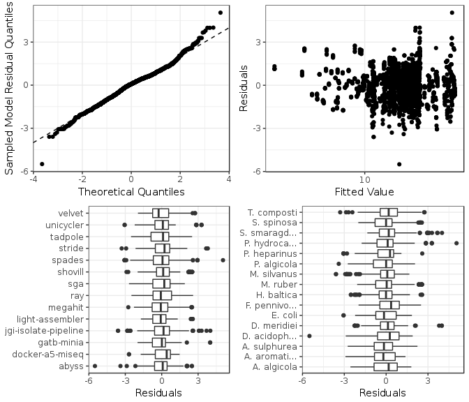
Figure 5: Model checking plots for NA50 fitted model. These are in clockwise order from upper left: comparison of model residual quantiles with theoretical quantiles, comparison of model residuals with fitted values, comparison of each assembler image model residuals, and comparison of each genome model residuals.
| Fixed Term | Random Term | Variance Model | dBIC | R.D.F. | Dev. | Conv. |
|---|---|---|---|---|---|---|
| Assembler | Genome | Assembler + Genome | 0.00 | 3697.049 | 6294.6 | F |
| Assembler Version | Genome | Assembler Version + Genome | 60.15 | 3677.045 | 6190.1 | F |
| Assembler | Genome | Genome | 104.18 | 3710.087 | 6506.1 | F |
| Assembler Version | Genome | Genome | 111.63 | 3700.091 | 6431.2 | F |
| Assembler Args | Genome | Genome | 153.57 | 3675.072 | 6267.2 | F |
| Assembler | Genome | Assembler | 1103.61 | 3712.106 | 7522.1 | F |
Table 3: Summary of first six most parsimonious models with number of misassemblies as the response variable. The dBIC shows the difference in Bayesian information criterion between the best model and all other models. ‘R.D.F.’ is the residual degrees of freedom in the model. ‘Dev.’ is the residual deviance in the model. ‘Conv.’ states whether the model converged or not (T/F).
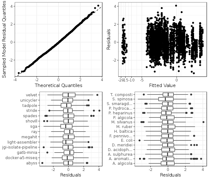
Figure 6: Model checking plots for misassemblies fitted model. These are in clockwise order from upper left: comparison of model residual quantiles with theoretical quantiles, comparison of model residuals with fitted values, comparison of each assembler image model residuals, and comparison of each genome model residuals.
| Fixed Term | Random Term | Variance Model | dBIC | R.D.F. | Dev. | Conv. |
|---|---|---|---|---|---|---|
| Assembler Version | Genome | Assembler Version + Genome | 0.00 | 3677.119 | 8404.4 | F |
| Assembler | Genome | Assembler + Genome | 60.35 | 3697.110 | 8629.3 | F |
| Assembler Version | Genome | Assembler Version | 370.94 | 3692.037 | 8898.1 | F |
| Assembler | Genome | Assembler | 396.52 | 3712.045 | 9088.4 | F |
| Assembler Version | Input FASTA | Assembler Version | 841.36 | 3629.771 | 8856.0 | F |
| Assembler | Input FASTA | Assembler | 873.33 | 3649.775 | 9052.6 | F |
Table 4: Summary of first six most parsimonious models with number of incorrect bases as the response variable. The dBIC shows the difference in Bayesian information criterion between the best model and all other models. ‘R.D.F.’ is the residual degrees of freedom in the model. ‘Dev.’ is the residual deviance in the model. ‘Conv.’ states whether the model converged or not (T/F).
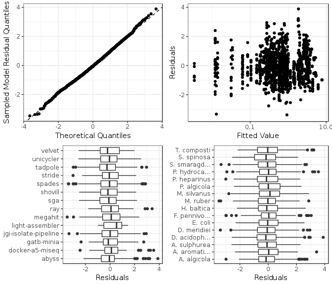
Figure 7: Model checking plots for incorrect bases model. These are in clockwise order from upper left: comparison of model residual quantiles with theoretical quantiles, comparison of model residuals with fitted values, comparison of each assembler image model residuals, and comparison of each genome model residuals.
| Fixed Term | Random Term | Variance Model | dBIC | R.D.F. | Dev. | Conv. |
|---|---|---|---|---|---|---|
| Assembler Args | Genome | Assembler Args + Genome | 0.00 | 3627.002 | 37732.5 | T |
| Assembler Args | Input FASTA | Assembler Args + Input FASTA | 1045.27 | 3499.044 | 37724.5 | F |
| Assembler Version | Genome | Assembler Version + Genome | 1461.26 | 3677.009 | 39605.3 | T |
| Assembler | Genome | Assembler + Genome | 2282.73 | 3697.007 | 40591.4 | T |
| Assembler Version | Input FASTA | Assembler Version + Input FASTA | 2421.13 | 3549.216 | 39513.3 | T |
| Assembler | Input FASTA | Assembler + Input FASTA | 3336.75 | 3569.135 | 40592.9 | F |
Table 5: Summary of first six most parsimonious models with L1 norm feature distance between reference and assembly as the response variable. The dBIC shows the difference in Bayesian information criterion between the best model and all other models. ‘R.D.F.’ is the residual degrees of freedom in the model. ‘Dev.’ is the residual deviance in the model. ‘Conv.’ states whether the model converged or not (T/F).
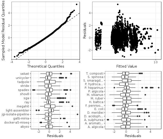
Figure 8: Model checking plots for feature L1 norm fitted model. These are in clockwise order from upper left: comparison of model residual quantiles with theoretical quantiles, comparison of model residuals with fitted values, comparison of each assembler image model residuals, and comparison of each genome model residuals.
| Fixed Term | Random Term | Variance Model |
|---|---|---|
| Null | Null | Null |
| Null | Genome | Null |
| Null | Genome | Genome |
| Null | Input FASTA | Null |
| Null | Input FASTA | Input FASTA |
| Assembler | Null | Null |
| Assembler | Null | Assembler |
| Assembler | Genome | Null |
| Assembler | Genome | Genome |
| Assembler | Genome | Assembler |
| Assembler | Genome | Assembler + Genome |
| Assembler | Input FASTA | Null |
| Assembler | Input FASTA | Input FASTA |
| Assembler | Input FASTA | Assembler |
| Assembler | Input FASTA | Assembler + Input FASTA |
| Assembler Version | Null | Null |
| Assembler Version | Null | Assembler Version |
| Assembler Version | Genome | Null |
| Assembler Version | Genome | Genome |
| Assembler Version | Genome | Assembler Version |
| Assembler Version | Genome | Assembler Version + Genome |
| Assembler Version | Input FASTA | Null |
| Assembler Version | Input FASTA | Input FASTA |
| Assembler Version | Input FASTA | Assembler Version |
| Assembler Version | Input FASTA | Assembler Version + Input FASTA |
| Assembler Args | Null | Null |
| Assembler Args | Null | Assembler Args |
| Assembler Args | Genome | Null |
| Assembler Args | Genome | Genome |
| Assembler Args | Genome | Assembler Args |
| Assembler Args | Genome | Assembler Args + Genome |
| Assembler Args | Input FASTA | Null |
| Assembler Args | Input FASTA | Input FASTA |
| Assembler Args | Input FASTA | Assembler Args |
| Assembler Args | Input FASTA | Assembler Args + Input FASTA |
Table 6: Comparison of the mixed effect models considered in this analysis, where each row defines the terms used in the model. The ‘Fixed’ and ‘Random’ terms are those fitted as explanatory variables, along with the natural log of the genome length. The ‘Variance Model’ column lists where the variance was also modelled as a component, i.e. whether different terms had different variances. Null terms indicate that this was simply modelled as the mean of the data with a model estimated constant coefficient.
| Assembler | Version | Task | #Incomplete |
|---|---|---|---|
| stride | 0.0.1-preprocessing | isolate | 74 |
| stride | 0.0.1-preprocessing | single-cell | 64 |
| velvet | 1.2.0 | default | 11 |
| tadpole | 36.38 | careful | 5 |
| tadpole | 36.38 | default | 5 |
| stride | 0.0.1-preprocessing | default | 2 |
| shovill | 0.2 | default | 1 |
| shovill | 0.7.1 | default | 1 |
| stride | 0.0.1 | default | 1 |
Table 7: List of biobox images failing to produce an assembly when run on benchmarking data.
| Assembler | Version |
|---|---|
| abyss | 2.0.1 |
| docker-a5-miseq | 20160825 |
| gatb-minia | 20161208-a4c6e8c |
| jgi-isolate-pipeline | v0.10.0 |
| jgi-isolate-pipeline | v0.11.0 |
| jgi-isolate-pipeline | v0.12.0 |
| light-assembler | 20161003-ed93715 |
| megahit | 1.0.6 |
| megahit | 1.1.1 |
| ray | 2.3.0 |
| sga | v0.10.13 |
| shovill | 0.2 |
| shovill | 0.4 |
| shovill | 0.7.1 |
| spades | 3.10.0 |
| spades | 3.10.1 |
| spades | 3.11.0 |
| spades | 3.11.0-fix-merge-task |
| spades | 3.9.0 |
| stride | 0.0.1 |
| stride | 0.0.1-preprocessing |
| tadpole | 36.38 |
| unicycler | v0.4.1 |
| velvet | 1.2.0 |
Table 8: List of biobox short read assembler Docker images used in the benchmarks.
| Biological Source | Length (MBp) | %GC |
|---|---|---|
| Algiphilus aromaticivorans | 3.81 | 66.38 |
| Amycolatopsis sulphurea | 6.86 | 69.41 |
| Arenibacter algicola | 5.55 | 39.74 |
| Desulfosporosinus acidophilus | 4.99 | 42.11 |
| Desulfosporosinus meridiei | 4.87 | 41.78 |
| Escherichia coli | 4.64 | 50.79 |
| Fervidobacterium pennivorans | 2.17 | 38.88 |
| Hirschia baltica | 3.54 | 45.19 |
| Meiothermus ruber | 3.10 | 63.38 |
| Meiothermus silvanus | 3.72 | 62.72 |
| Pedobacter heparinus | 5.17 | 42.05 |
| Polycyclovorans algicola | 3.65 | 63.78 |
| Porticoccus hydrocarbonoclasticus | 2.47 | 53.07 |
| Saccharopolyspora spinosa | 9.02 | 67.95 |
| Spirochaeta smaragdinae | 4.65 | 48.97 |
| Thermobacillus composti | 4.36 | 60.12 |
Table 9: List of source microbial genomes used in the benchmarks.
References
1. Earl DA, Bradnam K, St. John J, Darling A, Lin D, Faas J, et al. Assemblathon 1: A competitive assessment of de novo short read assembly methods. Genome Research. Cold Spring Harbor Laboratory Press; 2011;21: 2224–2241. doi:10.1101/gr.126599.111
2. Bradnam KR, Fass JN, Alexandrov A, Baranay P, Bechner M, Birol I, et al. Assemblathon 2: Evaluating de novo methods of genome assembly in three vertebrate species. GigaScience. 2013;2: 10+. doi:10.1186/2047-217x-2-10
3. Salzberg SL, Phillippy AM, Zimin A, Puiu D, Magoc T, Koren S, et al. GAGE: A critical evaluation of genome assemblies and assembly algorithms. Genome research. Cold Spring Harbor Laboratory Press; 2012;22: 557–567. doi:10.1101/gr.131383.111
4. Sczyrba A, Hofmann P, Belmann P, Koslicki D, Janssen S, Dröge J, et al. Critical assessment of metagenome interpretation-a benchmark of metagenomics software. Nature methods. 2017;14: 1063–1071. doi:doi:10.1038/nmeth.4458
5. Belmann P, Dröge J, Bremges A, McHardy AC, Sczyrba A, Barton MD. Bioboxes: Standardised containers for interchangeable bioinformatics software. GigaScience. 2015;4. doi:10.1186/s13742-015-0087-0
6. Gurevich A, Saveliev V, Vyahhi N, Tesler G. QUAST: Quality assessment tool for genome assemblies. Bioinformatics (Oxford, England). Oxford University Press; 2013;29: 1072–1075. doi:10.1093/bioinformatics/btt086
7. Simpson JT, Wong K, Jackman SD, Schein JE, Jones SJ, Birol I. ABySS: A parallel assembler for short read sequence data. Genome research. Cold Spring Harbor Laboratory Press; 2009;19: 1117–1123. doi:10.1101/gr.089532.108
8. Coil D, Jospin G, Darling AE. A5-miseq: An updated pipeline to assemble microbial genomes from Illumina MiSeq data. Bioinformatics (Oxford, England). Oxford University Press; 2015;31: 587–589. doi:10.1093/bioinformatics/btu661
9. Chikhi R, Rizk G. Space-efficient and exact de Bruijn graph representation based on a Bloom filter. Algorithms for molecular biology : AMB. 2013;8: 22+. doi:10.1186/1748-7188-8-22
10. El-Metwally S, Zakaria M, Hamza T. LightAssembler: Fast and memory-efficient assembly algorithm for high-throughput sequencing reads. Bioinformatics (Oxford, England). Oxford University Press; 2016;32: 3215–3223. doi:10.1093/bioinformatics/btw470
11. Li D, Liu C-MM, Luo R, Sadakane K, Lam T-WW. MEGAHIT: An ultra-fast single-node solution for large and complex metagenomics assembly via succinct de Bruijn graph. Bioinformatics (Oxford, England). Oxford University Press; 2015;31: 1674–1676. doi:10.1093/bioinformatics/btv033
12. Li D, Luo R, Liu C-MM, Leung C-MM, Ting H-FF, Sadakane K, et al. MEGAHIT v1.0: A fast and scalable metagenome assembler driven by advanced methodologies and community practices. Methods (San Diego, Calif). 2016;102: 3–11. doi:doi.org/10.1016/j.ymeth.2016.02.020
13. Boisvert S, Laviolette F, Corbeil J. Ray: Simultaneous assembly of reads from a mix of high-throughput sequencing technologies. Journal of computational biology : a journal of computational molecular cell biology. 2010;17: 1519–1533. doi:10.1089/cmb.2009.0238
14. Bankevich A, Nurk S, Antipov D, Gurevich AA, Dvorkin M, Kulikov AS, et al. SPAdes: A new genome assembly algorithm and its applications to single-cell sequencing. Journal of computational biology : a journal of computational molecular cell biology. Mary Ann Liebert, Inc., publishers; 2012;19: 455–477. doi:10.1089/cmb.2012.0021
15. Huang Y-TT, Liao C-FF. Integration of string and de Bruijn graphs for genome assembly. Bioinformatics (Oxford, England). 2016;32: 1301–1307. doi:10.1093/bioinformatics/btw011
16. Wick RR, Judd LM, Gorrie CL, Holt KE. Unicycler: Resolving bacterial genome assemblies from short and long sequencing reads. PLoS computational biology. 2017;13. doi:10.1371/journal.pcbi.1005595
17. Zerbino DR, Birney E. Velvet: Algorithms for de novo short read assembly using de Bruijn graphs. Genome research. Cold Spring Harbor Laboratory Press; 2008;18: 821–829. doi:10.1101/gr.074492.107
18. Ghodsi M, Hill CM, Astrovskaya I, Lin H, Sommer DD, Koren S, et al. De novo likelihood-based measures for comparing genome assemblies. BMC research notes. 2013;6: 334+. doi:10.1186/1756-0500-6-334
19. Simão FA, Waterhouse RM, Ioannidis P, Kriventseva EV, Zdobnov EM. BUSCO: Assessing genome assembly and annotation completeness with single-copy orthologs. Bioinformatics (Oxford, England). Oxford University Press; 2015;31: 3210–3212. doi:10.1093/bioinformatics/btv351
20. Meader S, Hillier LW, Locke D, Ponting CP, Lunter G. Genome assembly quality: Assessment and improvement using the neutral indel model. Genome research. 2010;20: 675–684. doi:10.1101/gr.096966.109
21. Parks DH, Imelfort M, Skennerton CT, Hugenholtz P, Tyson GW. CheckM: Assessing the quality of microbial genomes recovered from isolates, single cells, and metagenomes. Genome research. Cold Spring Harbor Laboratory Press; 2015;25: 1043–1055. doi:10.1101/gr.186072.114
22. Phillippy AM, Schatz MC, Pop M. Genome assembly forensics: Finding the elusive mis-assembly. Genome biology. 2008;9: R55+. doi:10.1186/gb-2008-9-3-r55
23. Hunt M, Kikuchi T, Sanders M, Newbold C, Berriman M, Otto TD. REAPR: A universal tool for genome assembly evaluation. Genome biology. BioMed Central Ltd; 2013;14: R47+. doi:10.1186/gb-2013-14-5-r47
24. Florea L, Souvorov A, Kalbfleisch TS, Salzberg SL. Genome assembly has a major impact on gene content: A comparison of annotation in two bos taurus assemblies. PloS one. 2011;6. doi:10.1371/journal.pone.0021400
25. Vezzi F, Narzisi G, Mishra B. Reevaluating assembly evaluations with feature response curves: GAGE and assemblathons. PloS one. Public Library of Science; 2012;7: e52210+. doi:10.1371/journal.pone.0052210
26. Schwarz G. Estimating the dimension of a model. The Annals of Statistics. 1978;6: 461–464. doi:10.1214/aos/1176344136
27. Burnham KP, Anderson DR. Multimodel inference. Sociological Methods & Research. SAGE Publications; 2004;33: 261–304. doi:10.1177/0049124104268644
28. Koren S, Phillippy AM. One chromosome, one contig: Complete microbial genomes from long-read sequencing and assembly. Current Opinion in Microbiology. 2015;23: 110–120. doi:10.1016/j.mib.2014.11.014
29. Burnham KP, Anderson DR. Model selection and multimodel inference: A practical information-theoretic approach. 2nd ed. Springer; 2002. pp. 1–488.
30. Stasinopoulos D, Rigby R. Generalized additive models for location scale and shape (gamlss) in R. Journal of Statistical Software, Articles. 2007;23: 1–46. doi:10.18637/jss.v023.i07
31. Shoukri MM. On the generalization and estimation for the double Poisson distribution. Springer-Verlag; 1982;33: 97–109. doi:10.1007/bf02888625
-
The linear models and linear mixed effects models in R (PDF) tutorial provides an explanation of why mixed effect models are used to model group level variance. In this case the group level variance is the source genome, and each individual observation is the FASTQ file given to the genome assembler.↩
-
As the free parameter penalty increases by the log of the number of observations, BIC has been described as a better choice than AIC for larger data sets [26], [27]↩
-
Based on suggested what to report when comparing models.↩
-
A given assembler estimated coefficient would added to a given genome estimated coefficient before being exponentiated to predict what the given metric should be for the genome. This is because the parameters are estimated as a linear model before being generalised with a log-normal link function to a Poisson 0-Inf distribution.↩
-
This does not use sequence alignment, but is instead a set operation. Does this exact annotation sequence in the reference also appear in the set of sequences annotated in the assembly? The L1 norm is the sum of these annotation differences between the reference and the assembly.↩