Examining microbial genome assemblies using contiguity metrics
An issue many researchers and analysts face is what is the best way to determine if a produced genome assembly is good or not, and by what criteria? Previous research has addressed this problem in assembly, including the Assemblathon 1 [1], Assemblathon 2 [2], GAGE [3], and CAMI [4]. The Joint Genome Institute faces the same problem on a larger scale. We’ve sequenced thousands of microbial genomes in the last five years and in every case we want to provide the best assembly given the available sequencing hardware, library preparation and assembly software. Over the last few years we have taken a two-fold approach to determine which assembly software to use.
-
Create Docker images with standardised interfaces to the majority of recent genome assembly software. This is the bioboxes project [5] in conjunction with Peter Belmann, and the other CAMI collaborators. The use of bioboxes allows the generated data to be useful to the microbial genomics community, since they can use exactly the same Docker image in their own research as was benchmarked.
-
Using increasing automation to evaluate larger numbers of these biobox genome assemblers against large amounts of Illumina microbial sequencing data where we also have a high quality reference genome as a ground truth for benchmarking. The use of large numbers of data sets allows for the identification of trends averaged over all observations. The aim being to remove any individual genome or sequencing specific effects when determining the effectiveness of an assembler.
Contiguity is often used to discuss the assembly quality. Specifically, this is how complete is the assembled sequence and how many separate fragments or ‘contigs’ there are. The most common measures of contiguity are L*50 and N*50 where * represents having zero or more of the characters in the set {g,a}. The N50 metric, originally described1 in the human genome paper [6], is calculated in the following steps:
-
Order in ascending order all contigs in the assembly by their length.
Calculate a running cumulative sum of the contig lengths
-
Find the pivot point in the cumulative sum that corresponds to half the total sum.
-
Pick the first contig that is greater than (specifically not greater and equal to) this halfway point in this running cumulative sum. The length of this contig is the value returned as the calculated N50 metric.
This is the N50 metric. All the N*50 and L*50 metrics in this analysis were estimated by comparing the assembly to the reference genome using QUAST [7], including:
-
NG50: Instead of using the halfway of point of the cumulative sum to find the pivot in the assembly, use half the sum of the reference assembly length. This prevents extraneous or duplicated contigs falsely inflating the N50 value. The NG50 metric was first defined in the Assemblathon 1 paper [1].
-
NA50: Before calculating N50, select only the contigs that map to the reference genome using alignment software. QUAST uses MUMmer for alignment [8]. Aligning the contigs prevents inflating the N50 value with contigs that should not be part of the assembly, such as contaminants or very poorly assembled regions.
-
NGA50: a combination of both of the above. Select only the contigs that map to the reference, and use half the sum of the reference assembly length as the pivot point. This is the strictest method of calculating N50. Both NA50 and NGA50 were defined by the QUAST team [7].
The L*50 metrics are calculated using the same method, but return instead the 1-based index of the contig. Starting at 1, the contigs are assigned an incrementing index until the first contig greater than the pivot. The index of this contig is the value of the L50 metric and represents the number of contigs which contain about half the assembly. All the N*50 variants described above have the corresponding L*50 metric. Keith Bradnam however has a detailed blog post about why the N50 metrics are useful [3].
The data I’m using here is a snapshot from a few months ago. You can download this data for yourself, and this article is also an RMarkdown document containing all the steps used to analyse the data. You can view the source or submit a pull request through the gitlab repository.
Exploration of contiguity metrics
Given all the metrics collected across ~6.5k genome assemblies in the nucleotid.es benchmarking project different, an exploratory first step is to determine if there are any obvious trends in these metrics across genomes and assemblers. Principal Components Analysis (PCA) is a common choice for the exploration of multivariate data because it allows projecting a multi-dimensional space into a lower two dimensional space which is then more easily visualised. Prior to performing PCA, metrics across all assemblies were preprocessed in the following way:
-
Any missing values were converted to 0. Missing values may be observed if the sum of contigs in an assembly are less the half the reference genome length, and therefore any *G50 metric cannot be calculated.
-
Each of the metrics: N*50 metrics, misassemblies and total length were scaled by the corresponding reference genome length, studentised to have a mean of 0, and to have a standard deviation of 12. This is to prevent the magnitude of the variable being the main component in the data.3
Figure 1 below visualises the first two principal components using these scaled contiguity metrics. The loadings of each of the contiguity metrics are shown as the vectors on the plot. The length of each vector shows how much variance is explained, and the angle between any two shows how much a given variable correlates with another in the same component.
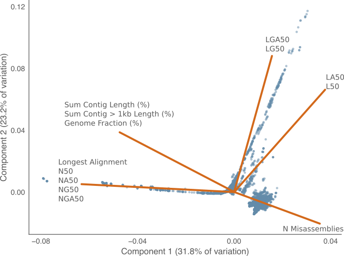
Figure 1: First two principal components for the variation in contiguity metrics across genome assemblies. Each point represents a single genome assembly from the nucleotid.es data set. The lines represent the loadings of each metric in the two principal components. The amount of variance explained by each component in listed the corresponding axis. Closely related loadings were grouped together for clarity.
The sum of first two components in PCA plot explains 55% of the variance in the assembly metric correlation matrix. In this subset of the explained variance, the most visible trend is the orthogonal relationship between the {L50, LA50, LG50, LGA50} metrics and the {N50, NG50, NA50, NGA50} metrics. I.e. these two groups of metrics likely have an inverse relationship.
A second observable trend is that the {L50, LA50} and {LG50, LGA50} metrics separate into two slightly different directions. There is not however the same difference between the corresponding N50/NA50 and NG50/NGA50 metrics. This may be a variant of the pigeon hole principle4: because L50 is a discrete random variable and two contiguous genome assemblies might have the same value by chance simply due to the limited number of discrete values L50 can take when the assembly contiguity is very good. The choice of the pivot when calculating LG50 versus L50 may therefore have a larger effect at smaller values. N50 values on the other hand tend to be a very large numbers, in the tens of thousands and so is distributed more like a continuous variable.
Comparing assemblies by contiguity
After using PCA to identify which metrics contribute to the variation in assemblies, a next step is to focus on a subset of variables that appear to be orthogonal in explaining variation. Figure 2 selects two of these identified variables: LA50 on the x-axis and NA50 on the y-axis. This figure further highlights possible pigeon hole effect in LA50, where small (good-contiguity) values are clumped into discrete buckets along the \(x\)-axis, and each of these buckets has a range of NA50 values along the \(y\)-axis. This trend is not apparent at the lower right end of the plot where LA50 is larger and more continuous. This figure also shows a general trend where LA50 and NA50 are anti-correlated at values associated with good-contiguity genome assemblies, but does not hold for poor-contiguity genome assemblies. Specifically in the upper left of the plot there is a linear relationship, while in the lower right in the range of values where L50 is greater than 100 indicating a poor assembly, the linear relationship no longer holds.
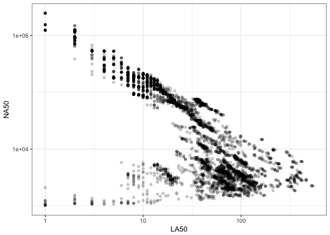
Figure 2: Comparison of genome assemblies by LA50 and NA50 metrics. Each point is a single genome assembly from the nucleotid.es data set.
The sequencing data used here for benchmarking were produced from two types of methods for extracting DNA: cultured colony isolates and multiple displacement amplification [9]. The first, isolate DNA, is extracted from a large number of microbial cells forming a colony. DNA can usually be generated in abundance with this method. Multiple displace amplification (MDA) data is often extracted from a single cell, and relies on polymerase chain reaction (PCR) amplification of the genome through random hexamer priming. The non-deterministic nature of the hexamer amplification means the entire genomic DNA might not be extracted, but only a fraction instead. We might anticipate that the random nature of which parts of the genome are extracted in MDA data has a strong effect on the resulting contiguity of the assembly, and therefore should not be treated the same as isolate data. We can examine this by repeating Figure 2 but highlighting the method used to extract the DNA.
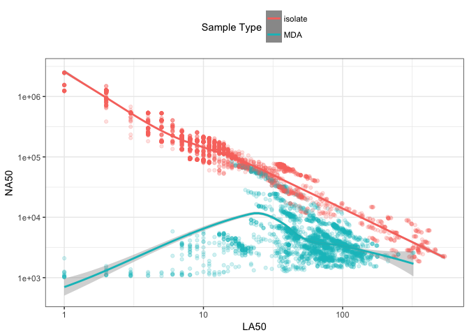
Figure 3: Comparison of genome assembly LA50 and NA50 metrics coloured by DNA extraction method. Each point is a single genome assembly from the nucleotid.es data set. Trending lines are added using loess smoothing.
Figure 3 shows a bipartite distribution between the colony-isolated and the MDA assemblies. The colony-isolated data shows a clear inverse relationship between the NA50 and LA50 metrics, while the MDA data shows no relationship. This indicates that the type of DNA extraction method has a significant effect on whether any conclusions can be drawn about the contiguity of an assembly based on N*50 or L*50 metrics. To put this another way, N*50 and L*50 metrics may be useful for examining colony-isolated assemblies for contiguity but, as is already generally accepted [10], MDA data breaks many of the assumptions used for assessing the quality of isolate assembled genomes.
Comparing assemblies across genomes
The N*50 family of metrics are not suitable for comparing assemblies between organisms with different genome sizes. To illustrate this, consider two genomes A and B, where the length of genome A is 100Mbp and the length of genome B is 10Mbp. The lengths of the contigs for the genome assembly A’ are {40, 30, 20, 10} and the lengths of the contigs for genome assembly B’ are {4, 3, 2, 1}. If we use N50 to compare these two genomes, then N50 for A’ is 40 while the N50 for B’ is 4. We might say that A’ is a more contiguous assembly than B’ because the N50 is higher for A’, however we know that this is an artefact of the length of the originating genome. Dividing both of these metrics by the length of the genome returns the value of 0.4 comparing both assemblies on the same scale.
When comparing the assemblies from two different genomes, the size of the genome is a component in the N*50 value. Therefore, it may be useful to define a metric based on N50, but divided by the originating genome length: NS50. For the purpose of this analysis any N*S50 metric is the corresponding N*50 metric divided by the sum of the reference genome contigs. The reason for doing so is when comparing genome assembly software we want to compare across a variety of different genomes, of unequal sizes. The signal we wish to identify is how well an assembler performs, and not any factors of the original genome size. Converting N*50 metrics into N*S50 metrics allows assemblies from two different genomes to be compared because these metrics are now invariant of the original genome length.5
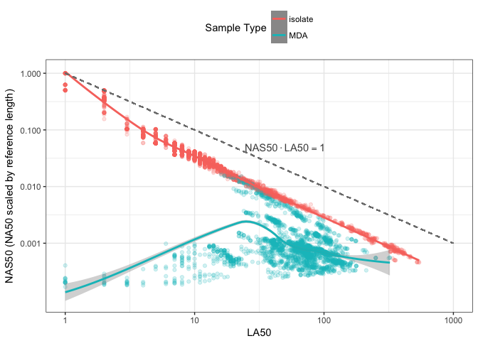
Figure 4: Comparison of LA50 and NA50 scaled by reference genome length. Each point is a single genome assembly from the nucleotid.es data set coloured by DNA extraction method. Trending lines are added using loess smoothing.
Using NS*50 metric, Figure 4 is the same as Figure 3 but using NAS50, the scaled version of NA50. The y-axis shows NAS50, the x-axis shows LA50, the colour of each point is the extraction method. Figure 4 is the most significant of this discussion, because it highlights the inverse relationship between NAS50 and LA50 for colony-isolated data, with much less variance in the relationship compared with Figure 3. The dashed line in the plot highlights the theoretical limit where LA50 metric cannot be any greater than 1, and when NA50 is scaled by the reference genome it also cannot be smaller than 1. A point (1,1) in the upper left therefore represents the perfect genome assembly, while values along this line LA50 \(\cdot\) NAS50 = 1 such as (10, 0.1), (100, 0.01) indicate progressively less contiguous assemblies. The product of all these values is still however 1.
The dashed line in Figure 4 appears to be an upper-bound on the product of these two metrics rather than a trend for colony-isolated assemblies. Specifically colony-isolated assemblies in Figure 4 fall below this line rather than around it. Figure 5 compares this distribution of LA50 \(\cdot\) NAS50, and shows a bimodal distribution. MDA data is associated with much smaller values of LA50 \(\cdot\) NAS50, which is not unexpected given that the size and quality of the genome assembled will strongly depend on lysis, and how much of the source material was amplified.
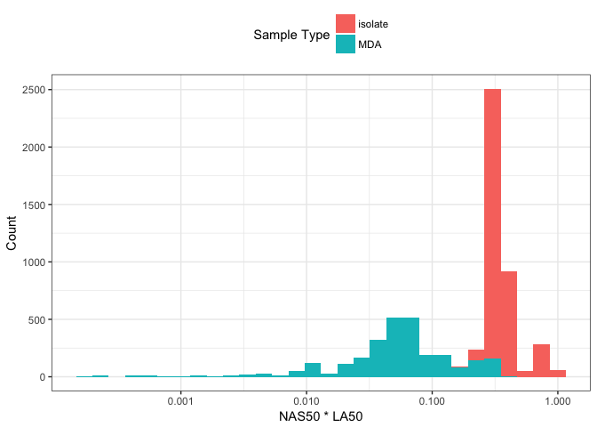
Figure 5: Histogram of NAS50 * LA50 distribution. Data are coloured by DNA extraction method.
Figure 6 compares NS50 \(\cdot\) L50 on the x-axis with percent genome fraction on the y-axis. Genome fraction is defined by QUAST as the percentage of bases aligned to the reference genome. The figure shows these two variables are correlated for MDA data, with an upper limit at (NS50 \(\cdot\) L50 \(\sim 10^{-\frac{1}{2}}\), 1) as highlighted by the dashed line. An interesting possibility may be if you can accurately estimate the size of the originating genome, it would be possible to determine percentage genome fraction for MDA data using NS50 \(\cdot\) L50 without having the reference genome to align against. For isolates, estimating a genome size without a genome should be possible from peaks in the sequencing kmer histogram.
The colony-isolated data shows no relationship between percentage genome fraction and NS50 \(\cdot\) L50. This suggests for isolates that most of the genome ends up in the assembly where the estimated genome fraction is at ~100%, but with varying degrees of contiguity along the NS50 \(\cdot\) L50 axis. This is as might be expected given that assemblies from colony-isolated microbial DNA should have most of the genomic DNA present.
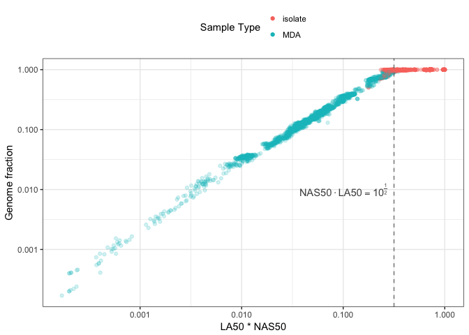
Figure 6: Comparison of NAS50 * LA50 with percent genome fraction. Genome fraction is the percentage of aligned bases to the reference genome as estimated by QUAST. A theoretical limit between isolate and MDA assemblies is shown by the dashed line.
Contiguity is only one aspect of an assembly
I attended the CAMI2 and M3 workshop in 2017 and was fortunate to see Mihai Pop give a talk on “Metagenome assembly and validation”. One of the points he discussed was that it is not enough to consider assembly contiguity alone, because large contiguous assemblies can be created by liberally introducing misassemblies. I.e. longer contigs may be generated by incorrectly assembling difficult genomic regions. Therefore it’s worth measuring the extent to which contiguity and misassemblies are inversely correlated.
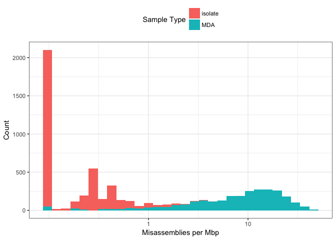
Figure 7: Distribution of misassemblies across genome assemblies, coloured by DNA extraction method.
Figure 7 shows the distribution of number of misassemblies per megabase across the data. A small value (0.1) was added to 0 values to visualise them on a log10 scale. This figure shows, as might be expected given chimeric reads and very uneven coverage, that MDA data has a much greater number of misassemblies than colony-isolated data. The number of misassemblies in MDA data ranges over two orders of magnitude.
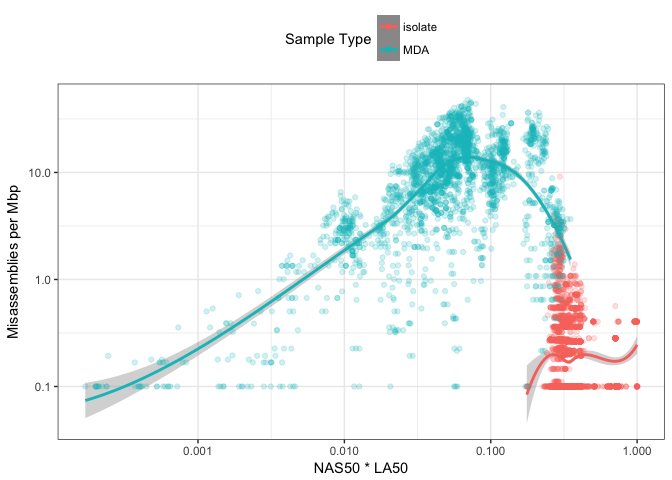
Figure 8: Comparison of NAS50*LA50 with number of misassemblies per megabase. Trending lines are added using loess smoothing.
Figure 8 compares the distribution of misassemblies on the y-axis and NS50 \(\cdot\) L50 on the x-axis. This indicates there is no readily-observable relationship between the contiguity of an assembly and the number of misassemblies. This is particularly the case for the colony-isolated data. The MDA data might suggest some relationship but given the density and spread of the data, there is no trend I would trust to use as a metric for evaluating the number of misassemblies. I think this reinforces Mihai Pop’s point that contiguity metrics alone are not enough to identify the quality of an assembly, and methods for identifying misassemblies should also be used too.
Summary
-
When examining the contiguity of a microbial assembly using a subset of the metrics produced by QUAST. The N*50 and L*50 metrics are near orthogonal in describing 55% of the variation identified in the first two principal components.
-
When N*50 metrics are scaled by the length of the originating microbial genome (as N*S50), then L*50 and N*50 are inversely proportional in culture-colony isolated microbial DNA, such that there appears to be an upper limit at NS50 \(\cdot\) L50 = 1.
-
The relationship NS50 \(\cdot\) L50 = 1 does not hold for multiple displacement amplification isolated microbial DNA, likely because not all of the genomic DNA will be extracted due to the stochastic nature of the process. The value NS50 \(\cdot\) L50 may however be useful for determine the percentage of the genome in an MDA assembly, if the size of the genome can be estimated.
-
Microbial contiguity metrics show little relationship with the amount of misassembled regions, particularly so with colony-isolated DNA assemblies. Contiguity metrics alone should not be used to benchmark a microbial genome assembler. Tools such as reapr [11] and VALET [12] may be helpful to identify misassemblies.
Acknowledgements
The work was conducted at the U.S. Department of Energy Joint Genome Institute, a DOE Office of Science User Facility, and is supported under Contract No. DE-AC02-05CH11231. Multiple instances of advice and suggestions provided on Cross Validated to make the model fitting part of this analysis possible.
Postscript - evaluation of reference-free metrics
The ideal metrics to benchmark the contiguity of an assembly would be LGA50 and NGA50 because this pivot for calculating the metric is length of reference rather than the length of assembly which may contain spurious or misassembled contigs. Excluding any contigs that do not align to the reference also removes parts of the assembly that have low sequence similarity. Without a reference however, it is only possible to calculate L50 and N50 respectively. Figure 9 therefore compares N50/NGA50 and L50/LGA50 respectively to determine the correspondence between the reference-based and non-reference-based metrics.
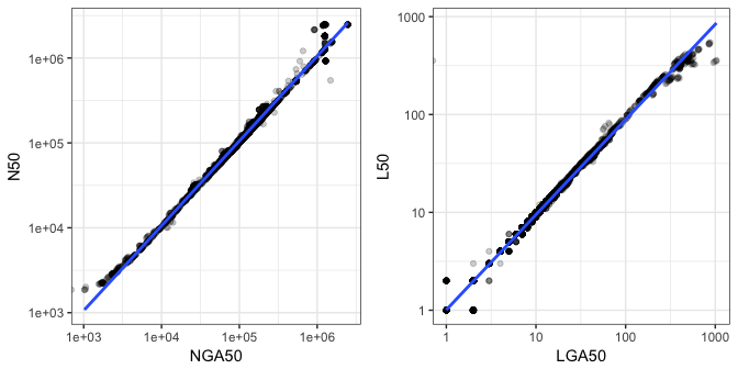
Figure 9: Comparison of reference-based assembly contiguity metrics with non-reference-based counterparts. Only colony isolated genome assemblies are plotted. Trend lines are added using a linear model.
Figure 9 indicates there is good correspondence between these two sets of metrics, therefore you might assume that L50 is a good proxy for LGA50, and N50 correspondingly for NGA50. This however does come with the caveat, that the two plots above were generated using only colony-isolated data. It’s not possible to calculate NG50 when the size of the assembly is less than 50% the length of the reference as is common in MDA data. Contiguity metrics should therefore be used with even more caution on MDA data. This may also hold true for metagenome assemblies, which if complex enough and without enough sequencing depth, would also not contain 50% the length of the original genomes.
References
1. Earl DA, Bradnam K, St. John J, Darling A, Lin D, Faas J, et al. Assemblathon 1: A competitive assessment of de novo short read assembly methods. Genome Research. Cold Spring Harbor Laboratory Press; 2011;21: 2224–2241. doi:10.1101/gr.126599.111
2. Salzberg SL, Phillippy AM, Zimin A, Puiu D, Magoc T, Koren S, et al. GAGE: A critical evaluation of genome assemblies and assembly algorithms. Genome research. Cold Spring Harbor Laboratory Press; 2012;22: 557–567. doi:10.1101/gr.131383.111
3. Bradnam KR, Fass JN, Alexandrov A, Baranay P, Bechner M, Birol I, et al. Assemblathon 2: Evaluating de novo methods of genome assembly in three vertebrate species. GigaScience. 2013;2: 10+. doi:10.1186/2047-217x-2-10
4. Sczyrba A, Hofmann P, Belmann P, Koslicki D, Janssen S, Dröge J, et al. Critical assessment of metagenome interpretation-a benchmark of metagenomics software. Nature methods. 2017;14: 1063–1071. doi:doi:10.1038/nmeth.4458
5. Belmann P, Dröge J, Bremges A, McHardy AC, Sczyrba A, Barton MD. Bioboxes: Standardised containers for interchangeable bioinformatics software. GigaScience. 2015;4. doi:10.1186/s13742-015-0087-0
6. Initial sequencing and analysis of the human genome. Nature. Nature Publishing Group; 2001;409: 860–921. doi:10.1038/35057062
7. Gurevich A, Saveliev V, Vyahhi N, Tesler G. QUAST: Quality assessment tool for genome assemblies. Bioinformatics (Oxford, England). Oxford University Press; 2013;29: 1072–1075. doi:10.1093/bioinformatics/btt086
8. Kurtz S, Phillippy A, Delcher AL, Smoot M, Shumway M, Antonescu C, et al. Versatile and open software for comparing large genomes. Genome Biology. Center for Bioinformatics, University of Hamburg, Bundesstrasse 43, 20146 Hamburg, Germany.: BioMed Central Ltd; 2004;5: R12+. doi:10.1186/gb-2004-5-2-r12
9. Spits C, Le Caignec C, De Rycke M, Van Haute L, Van Steirteghem A, Liebaers I, et al. Whole-genome multiple displacement amplification from single cells. Nature protocols. Research Centre Reproduction; Genetics, Academisch Ziekenhuis, Vrije Universiteit Brussel, Brussels, 1090, Belgium. 2006;1: 1965–1970. doi:10.1038/nprot.2006.326
10. Chitsaz H, Yee-Greenbaum JL, Tesler G, Lombardo M-JJ, Dupont CL, Badger JH, et al. Efficient de novo assembly of single-cell bacterial genomes from short-read data sets. Nature biotechnology. Nature Publishing Group; 2011;29: 915–921. doi:10.1038/nbt.1966
11. Hunt M, Kikuchi T, Sanders M, Newbold C, Berriman M, Otto TD. REAPR: A universal tool for genome assembly evaluation. Genome biology. BioMed Central Ltd; 2013;14: R47+. doi:10.1186/gb-2013-14-5-r47
12. Hill CM. Novel methods for comparing and evaluating single and metagenomic assemblies [Internet]. PhD thesis. 2015. Available: https://drum.lib.umd.edu/handle/1903/17100
-
Keith Bradnam describes the origins of the term N50 with an interesting blog post.↩
-
Scaling a variable to have a mean of 0, and a standard deviation of 1 converts the variable to a z-score.↩
-
PCA projects into the dimensions which maximise the variance. Scaling prevents the magnitude of the variable being the main component. Converting all the contiguity metrics into their z-score values is therefore the same as performing PCA on the correlation matrix rather than covariance matrix.↩
-
The pigeon hole principal describes when binning a limited number of values into a limited number of bins, then some values will be the same. For example putting 10 pigeons into 9 holes, then at least one hole will have two pigeons.↩
-
The L*50 metrics are invariant of size since they are calculated as the number of contigs. I think it could be argued that larger genomes are likely to have more difficult regions to assemble, therefore resulting in a higher L*50 value. My unproven intuition however is that dividing L50 would introduce a much greater reference length bias than simply leaving the metric as is. An additional point is that NS50 is a scale-free metric, as is L50 and therefore makes these metrics comparable also.↩